
2026 Mid-Year Forecast
#308 | The top-3 analogs and the Gann annual cycle method, testing against the August and September windows from #306.

Introduction
In my post #306, I listed two dates for the back half of 2026: August 8 and September 23, the two that carry the most weight in Gann’s seasonal record. I said then that whether either becomes a real turning point depends on what the cycle hierarchy and the analogs indicate once I run them. This is an update on the two independent studies: the top-3 analog correlations and the Gann annual cycle method.
As you remember, a reader pushed back in May against my continued use of the 60-year cycle analogy. His read was that the 60-year cycle has been off track since 2022, and that changing the read along the way makes tracking it meaningless. I didn’t dismiss it. The 60-year cycle isn’t always the dominant one, and I’ve said so before. But it’s one cycle within a hierarchy, and the mid-year mark is the place to show that rather than argue it.
Gann had a line for the rest of it: “In Wall Street, the man who does not change his mind will soon have no change to mind” (Gann, 45 Years in Wall Street, 1949).
The lesson here for all of us: don’t hold on to a bias or a previous analysis when the odds turn against you.
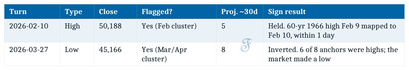
Here’s where the first half left us, to the day. The DJIA made a high of 50,188 on February 10, a low of 45,166 on March 27, and a new high of 51,562 on June 4. That last print ran past the 1966 forecast (inversion?) on which the second-half bias rested. I will start there, because it’s the true starting point.
Where the first half landed
Two turns were realized in the first half, and the Gann method had something to say about both. February held as a high, with the nearby cycle anchors reading high. Six of the eight Gann time cycles were projected from a past high but came in as lows by the end of March 2026: the 60-year cycle inverted across these turns. So the timing flagged both inflection points. You can’t draw a conclusion from two turns, and I’ll classify it as exactly that: thin.
Note: the tests show that inversions occur, as past highs and lows may change polarity over time.
The June 4 high is the one that matters for the second half of 2026. At 51,562, the index traded above the level the 1966 analog sat at, with that forecast pointing to an early-year high and an autumn low. The way I read this is that the 1966 price overlay is off the table for now.
The top-3 analogs, re-ranked
I built a tool that ranks past years by how closely each matches the current year’s pattern, weighted by correlation through June 12. It re-ranked the analogs using a January 2 to June 12 window (112 trading days).
The set now leads with three years: 1898 at r 0.78, 1890 at r 0.67, and 1978 at r 0.63.
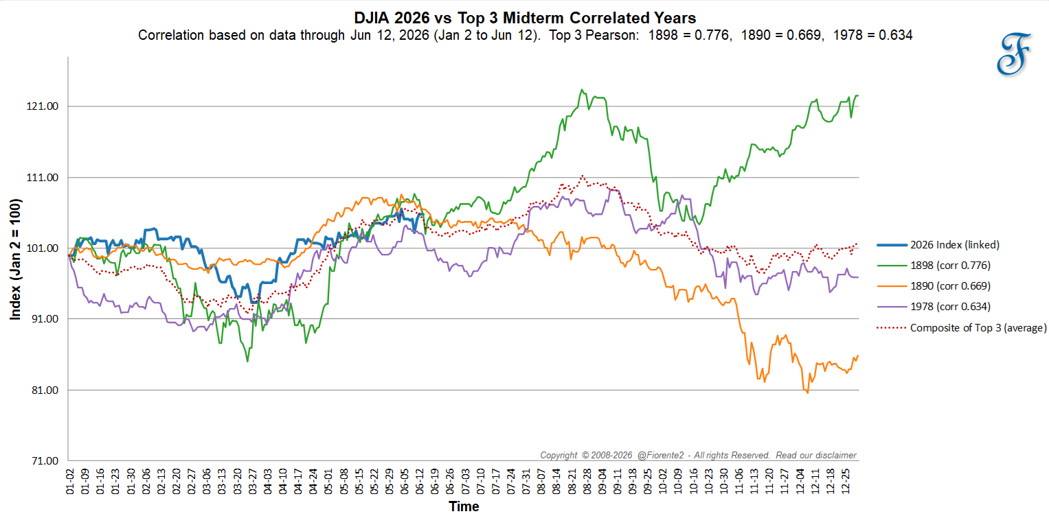
That’s a real change from spring. The April data was led by 1966, but 1966 has since slipped to rank 23, and 1926 dropped out of the top group. Only 1898 carried over from the April top three. The set shifted toward three older years.
Three analogs at r 0.6 and up are a reading worth weighing. It’s a small sample, and the index might not follow any of them. Cycles contract, extend, and invert.
The obvious objection is that an empirical correlation search and Gann’s fixed cycles are two different tools that may not agree.
Run the distances back from 2026, though, and they mostly do. 1978 is 48 years ago, which is 2 times the 24-year cycle, also 4 times 12, and it sits just under the 49-to-50-year Jubilee zone. 1890 is 136 years back, close to 3 times 45, which is near the Saturn-Uranus synodic cycle (45.33 years)1
So the correlation tool and Gann’s cycle projection nominate the same years from opposite ends: one by price fit, the other by time-cycle count.
1898 is the exception. It’s the strongest fit at r 0.78 and the loosest harmonic, the year the fixed cycles would never have nominated on their own, yet it still resonates on a similar theme.
When three years line up this closely, it’s worth looking into what happened in them.
These analog years agree on similar political and economic themes, each near a major tariff episode: the McKinley Tariff in 18902, the Dingley Tariff in 18973 into 1898 (which raised rates to protect manufacturers and factory workers from foreign competition), and the 1978 dollar crisis, inflation, and Japan trade friction through 19784.
All three years also printed an autumn low. The 1890 and 1978 cases continued lower into year-end lows, while 1898 made an October low and rallied to a new high by December.
The correlation doesn’t prove a tariff link, but it’s a condition that aligns.
What the Gann annual cycle method revealed.
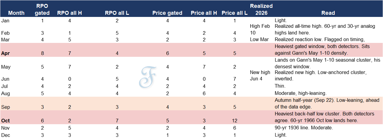
Before I make any call on a cycle window for the second half of 2026, I owe you the test I ran this month. The method projects all of Gann’s 33 cycles, from 90 years down to the minor 1-year cycle, forward, and watches for dates where many of them land at once: a cluster. The question I put to myself is whether a cluster marks a turn more often than chance.
I detrended the data and backtested it in 7 runs, using a relative price oscillator (RPO, which strips the trend) and the price level itself (the price detector), across 2022 and 2026, from monthly to weekly to daily, on the DJIA back to 1885, to test whether the timeframe makes a difference. A lift of 1.0 means the cluster did no better than the base rate; above 1.0 is an edge.
On the monthly timeframe, the DJIA sits within one month of a detrended turn about 23% of the time to begin with. The dense-cluster months lifted that to a 1.41 hit rate, and the edge held after a backtest split the range at 1960.
On the weekly timeframe, that edge washed out. In the flagged weeks, 9 of 222 sat on a turn: a 4.1% hit rate against a 4.1% base rate. A lift of 1.00, which is to say no edge at all.
On the daily timeframe, it scatters. The lift sits near 1.1 at every window and doesn’t sharpen as the window tightens. After 1960, it fell to about 1.05.
The tests show that a monthly chart is enough to mark a zone to watch where a high or low may land. More data points on a weekly or daily chart didn’t add an edge or sharpen the timing of cycle crests or troughs.
Testing the method on 2022, it caught the January 2022 high, the September and October lows, and the November 30 high. So far in 2026, the 1966 high echoed in February 2026, and we now know the March low inverted on a March/April cluster.
I summarized the 2022 and 2026 results in the table below:
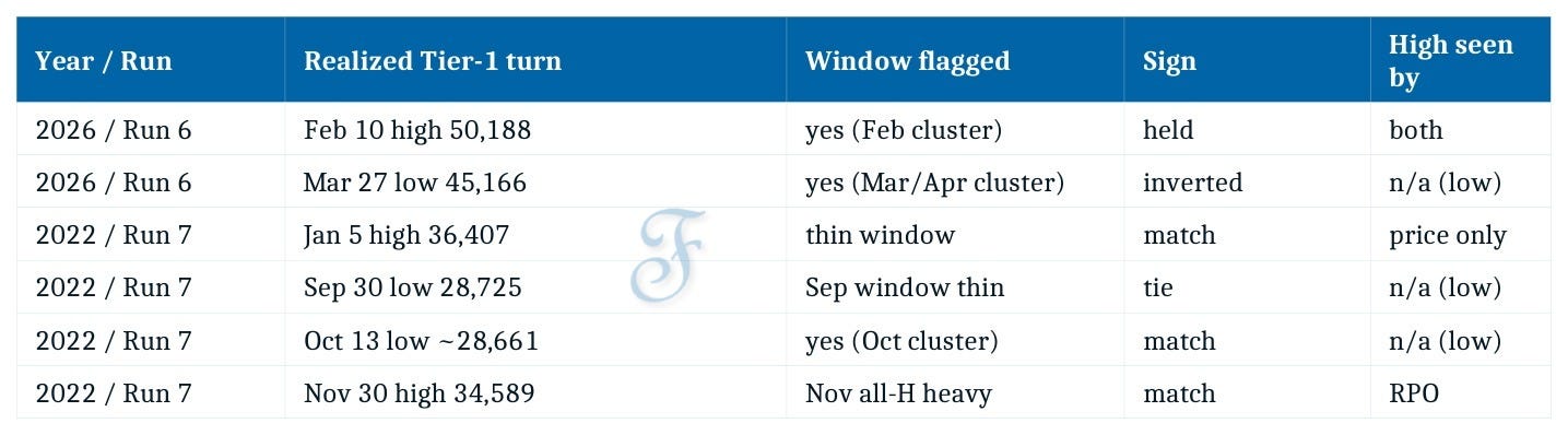
The table also shows which method, RPO or price detector, matched the actual high or low printed.
Gann never sold the annual forecast as foolproof, and the studies land where he did. He read the year as an analog that “will run very close to the last 10-year cycle,” then told you to “watch for minor variations in monthly moves” and to judge each stock on its own base (Gann, Master Stock Market Course, 1955, Rule 9).
He put the fallibility into the trading as much as the timing: “When making a trade, remember that you can be wrong or that the market may change its trend and the STOP LOSS order will protect you” (same source).
Note: the annual forecast was only one part of his method. In his day, he judged the public wasn’t ready for the astronomical cycles, so he called them time cycles and left a clue through the 30-year cycle, the Saturn cycle, which he named just once. My best guess is that he read the planetary cycles alongside the time cycles to judge how a year’s forecast would play out and which analogs would confirm it. Something for my further research.
A probable path into the year-end
Putting all of the recent research into perspective, here’s how the second half of 2026 may work out.
In post #306, I flagged August 8 and September 23 on the seasonal layer alone. With the hierarchy and the top-3 analogs run, here’s what supports each.
August 8 has picked up top-3 analog support. The top-3 composite recorded a low on August 7, one day off the seasonal date. So a date I flagged in May on seasonal weight alone now has the analog set behind it: a seasonal trigger and a composite-analog low in the same window. It’s never proof it will play out this way; it remains a probable forecast.
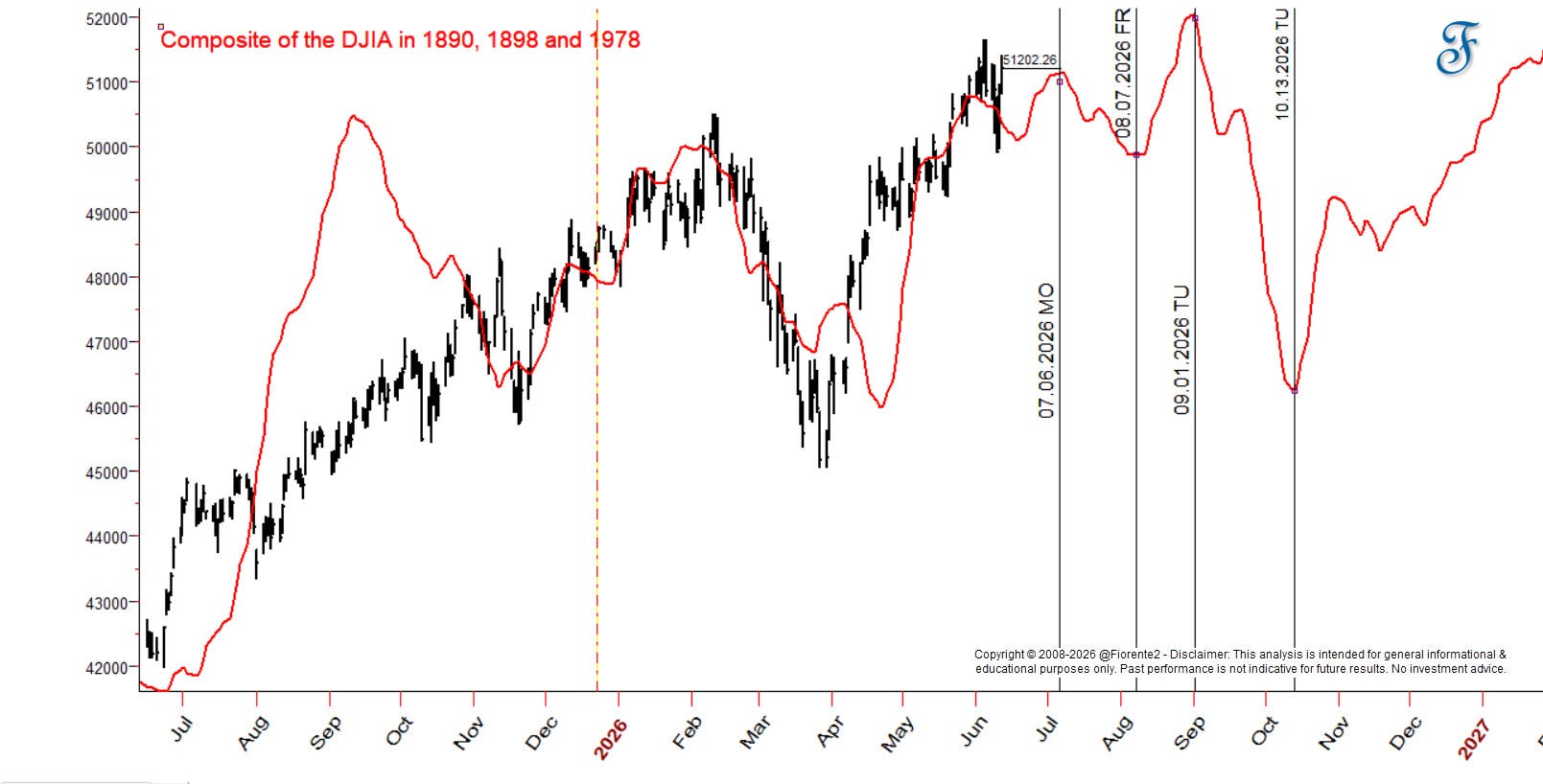
September 23 reads as a bracket rather than a hit. The composite shows a high on September 1 and a low on October 13, which places September 23 in the declining phase between them. The analog set points to continued weakness into that date, without pinpointing the exact day. Support holds through the period, with the turn marked on the chart.
October is where the cycles stack up, and it’s the strongest read in the forecast. The composite’s October 13 low falls within the cluster method’s heaviest second-half low window for 2026, with 5 of 6 clustered-cycle hits (the RPO) and 12 of 15 from the price detector.
The seasonal layer, the cluster method, and the analog top-3 composite all point to the late-September-into-October zone. The 60-year cycle’s timing lands here too. The 1966 price overlay is off after June 4, but the cycle’s turn date stays in the window, so like last year I’d give it more weight in the second half.
The 1936 March low (90-year) echoed in a March 2026 low, and that year ended with a high into early 1937. So 2026 may well end with a high. That’s the complexity we have to work with.
Where the cycles disagree, I keep the options open. Confirmation comes from the chart, not the calendar.
My preference for now is the composite path. From here it points to a July 6 high, an August 7 pullback low, a run-up to a September 1 high near 52,000, then a decline into an October 13 low near 46,200, with a recovery into year-end. These are probability windows, not exact dates.
The line that would close this path: a daily close above roughly 52,500 before the August window would mean the pullback didn’t arrive and tilt me to the 1898 case; a daily close below 46,200 before September would mean the decline ran early. Either way, I’ll update.
There’s an inversion case worth weighing. 1898 is the bullish exception in the top-3 set, and the June 4 break above the 1966 forecast suggests 2026 may be tracking a stronger analog.
If 1898 leads, the back half would hold its September high, and the autumn decline would come in shallower than the composite shows, or not at all.
Conclusion
Two windows stand out for the back half: the August 7-8 zone, now carried by both the seasonal date and the top-3 analog low, and the late-September-into-October zone, where three cycles agree on a low.
This is my bias for now: the composite path through both windows, with 1898 as the inversion case that would keep the market stronger for longer, similar to the 90-year cycle (the 1936 similarity). No advice.
Back to the reader who said the 60-year cycle went off track. He’s partly right, which is the point. No single cycle predicts everything. The 60-year is one cycle in the hierarchy. The cluster method gives a monthly watch window. The analog set re-sorts as the year goes on. These methods are worth most when they agree.
Remember, cycles can contract, extend, and invert. I may be wrong, of course. Anomalies can occur, fundamentals can shift, so be cautious.
In case you haven’t noticed, I post various charts in the Substack notes every week. You can find them all here. (click on the link)
P.S.: I’ll post the next update on the inflection points, or sooner if the path breaks early. Subscribers get it by email from the day they join. To follow all of my research and the 2026 forecast, subscribe for free.
If you liked this post from @Fiorente2’s Blog, why not restack and share it?
© 2008–2026 Fiorente2.com. All Rights Reserved.
Disclaimer: This analysis is for informational and educational purposes only and should not be considered investment advice. Read our full disclaimer.
Disclosure: From time to time, I may hold positions in the securities mentioned.
The Saturn-Uranus cycle, projected from the 1890 low, produced significant lows on 60-degree steps in October 1987, October 2002, March 2009, and April 2025. Perhaps on its way to an early 2032 low.